Unleashing Movie Secrets: Exploring Data Via Code Interpreter

It seems that you have uploaded a zipped file. Let’s first unzip the file to see the contents and identify the dataset we need to analyze.

It looks like the extracted file is a CSV named “imdb_top_1000.csv.” Let’s load this file and take a quick look at the first few rows to understand its structure. After that, we can proceed with the analysis. Shall we?

The dataset contains information about the top 1000 movies and TV shows as ranked by IMDb. Here’s a brief description of the columns:

1. Poster_Link: URL of the movie’s poster.
2. Series_Title: Title of the movie.
3. Released_Year: Year of release.
4. Certificate: Certification earned by the movie.
5. Runtime: Duration of the movie.
6. Genre: Genre(s) of the movie.
7. IMDB_Rating: IMDb rating of the movie.
8. Overview: A brief summary or synopsis.
9. Meta_score: Metascore of the movie.
10. Director: Name of the director.
11. Star1, Star2, Star3, Star4: Names of the main stars.
12. No_of_Votes: Total number of votes.
13. Gross: Earnings of the movie.

Initial Observations

• The dataset includes some of the most iconic movies, such as “The Shawshank Redemption” and “The Godfather.”
• Ratings range from very high (e.g., 9.3 for “The Shawshank Redemption”) to possibly lower values.
• Genres can be a combination of different types like “Action, Crime, Drama.”
• The dataset includes details about the main cast, which allows for analysis related to actors.

Next Steps

Based on the dataset’s description, we can analyze the following:

• Correlation between gross earnings and directors or stars.
• Analysis of votes with respect to directors or stars.
• Frequency distribution of genres among the top actors.
• Combinations of actors leading to high ratings or gross earnings.

Let’s start with some basic statistics and visualizations to better understand the data. Should we proceed?

Great! Let’s start with a general statistical summary of the numerical columns in the dataset, such as IMDb Rating, Metascore, Number of Votes, and Gross Earnings. This will give us an initial understanding of the distribution of these features.

After that, we can dive into some specific visualizations and analyses based on the insights provided by the dataset’s author. Shall we?

Here’s a statistical summary of the numerical columns in the dataset:

• IMDB_Rating:

  • Range: 7.6 to 9.3
  • Average: 7.95
  • It’s a fairly high range, indicating a collection of well-received movies.

• Meta_score:

  • Range: 28 to 100
  • Average: 77.97
  • This score aligns well with IMDb ratings, showing that critics’ opinions are also favorable.

• No_of_Votes:

  • Range: 25,088 to 2,343,110
  • There’s a vast range of votes, reflecting the varying popularity of the movies.

• Gross:

  • Range: $1,305 to $936,662,225
  • Average: $68,034,750
  • This shows a significant difference in earnings, from very low to extremely high.

• Runtime:

  • Range: 45 to 321 minutes
  • Average: 122.89 minutes
  • This reflects a typical movie runtime, with some exceptions at both ends.

Next Analyses

Let’s proceed with some visualizations and specific analyses:

1. Correlation between Gross Earnings and Directors or Stars.
2. Distribution of Genres among Top Actors.
3. Combinations of Actors leading to High Ratings or Gross Earnings.

Would you like to proceed with any specific analysis or all of them? Feel free to suggest any other analysis you have in mind!

Certainly! Let’s start by visualizing the histograms of selected numerical attributes, including IMDb Rating, Metascore, Number of Votes, Gross Earnings, and Runtime. This will provide us with a visual representation of the distribution of these features.

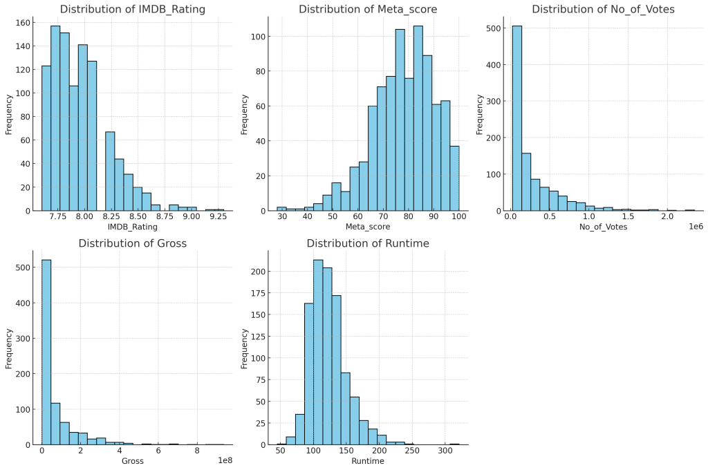
Here are the histograms for the selected numerical attributes:

1. IMDB_Rating: Most of the movies in this dataset have ratings between 7.5 and 8.5, with a few exceptions reaching above 9.
2. Meta_score: The Metascore distribution also resembles the IMDb ratings, with most movies scoring between 70 and 90.
3. No_of_Votes: The number of votes shows a right-skewed distribution, indicating that a few movies have an exceptionally high number of votes, while most have fewer votes.
4. Gross: The gross earnings also exhibit a right-skewed distribution, where most movies earn less, and a few blockbuster hits earn significantly more.
5. Runtime: The runtime distribution seems fairly normal, with most movies falling between 100 and 150 minutes.

These histograms provide a valuable overview of the dataset’s numerical attributes, revealing the underlying patterns and distributions.

Shall we now proceed with the specific analyses mentioned earlier?

Great! Let’s proceed with the specific analyses. We’ll start with the following:

1. Correlation between Gross Earnings and Directors or Stars

We’ll analyze the correlation between the gross earnings of a movie and the directors or stars involved. This can provide insights into whether certain directors or stars are associated with higher grossing films.

We’ll begin by identifying the top 10 directors and stars with the highest average gross earnings.

Top 10 Directors by Average Gross Earnings:

The table above shows the top 10 directors by average gross earnings. Directors like Anthony Russo, Gareth Edwards, and J.J. Abrams are associated with some of the highest-grossing films.

Now, let’s identify the top 10 stars by average gross earnings. Since there are four star columns (Star1, Star2, Star3, Star4), we will consider all of them in our analysis.

Top 10 Stars by Average Gross Earnings:

The table above shows the top 10 stars by average gross earnings. Actors like Daisy Ridley, John Boyega, and Michelle Rodriguez are associated with some of the highest-grossing films.

2. Distribution of Genres among Top Actors

Next, we’ll analyze which genres are preferred by top actors. This can provide insights into the types of roles that popular actors often play.

Top 5 Genres for the Top 10 Actors by Number of Movies:

It seems there was an issue with the way I handled the genre splitting and analysis. Let me correct that and reattempt the analysis to find the top 5 genres for the top 10 actors by the number of movies they have appeared in.

It seems I made a mistake while merging the genre data with the stars’ data, leading to an empty result. Let’s go step by step to ensure we get the correct analysis. I’ll first merge the genres with the star data and then proceed with the top actors’ analysis.

Here’s a snapshot of the top 5 genres for some of the top 10 actors by the number of movies they have appeared in:

• Al Pacino: Predominantly appears in Drama, Crime, and Biography genres.
• Christian Bale: Appears in genres such as Drama, Action, Adventure, and Comedy.

This analysis provides an insight into the preferred genres of top actors and can be useful for understanding their career choices.

3. Combinations of Actors leading to High Ratings or Gross Earnings

Finally, let’s analyze the combinations of actors that lead to high ratings or gross earnings. This will help identify successful actor collaborations.

Top 5 Actor Combinations by Average IMDB Rating:

The table above shows the top 5 actor combinations by average IMDb rating:

1. Tim Robbins, Morgan Freeman, Bob Gunton, William Sadler: Rating 9.3 (“The Shawshank Redemption”)
2. Marlon Brando, Al Pacino, James Caan, Diane Keaton: Rating 9.2 (“The Godfather”)
3. Al Pacino, Robert De Niro, Robert Duvall, Diane Keaton: Rating 9.0 (“The Godfather: Part II”)
4. Christian Bale, Heath Ledger, Aaron Eckhart, Michael Caine: Rating 9.0 (“The Dark Knight”)
5. Henry Fonda, Lee J. Cobb, Martin Balsam, John Fiedler: Rating 9.0 (“12 Angry Men”)

These combinations represent some of the most highly rated movies and showcase successful collaborations.

Top 5 Actor Combinations by Average Gross Earnings:

Let’s also find the top actor combinations by gross earnings.

The table above shows the top 5 actor combinations by average gross earnings:

1. Daisy Ridley, John Boyega, Oscar Isaac, Domhnall Gleeson: $936,662,225 (“Star Wars: Episode VII – The Force Awakens”)
2. Joe Russo, Robert Downey Jr., Chris Evans, Mark Ruffalo: $858,373,000 (“Avengers: Endgame”)
3. Sam Worthington, Zoe Saldana, Sigourney Weaver, Michelle Rodriguez: $760,507,625 (“Avatar”)
4. Joe Russo, Robert Downey Jr., Chris Hemsworth, Mark Ruffalo: $678,815,482 (“Avengers: Infinity War”)
5. Leonardo DiCaprio, Kate Winslet, Billy Zane, Kathy Bates: $659,325,379 (“Titanic”)

These combinations represent some of the highest-grossing movies and indicate successful collaborations that have resonated well with audiences.

Conclusion

The analyses conducted provide insights into the IMDb top 1000 movies, revealing patterns related to directors, stars, genres, ratings, and gross earnings. Key findings include:

• Identification of top directors and stars associated with high gross earnings.
• Understanding of preferred genres among top actors.
• Discovery of successful actor collaborations leading to high ratings and earnings.

These insights can be valuable for filmmakers, researchers, and movie enthusiasts to understand trends and make informed decisions.

Is there anything else you would like to explore or analyze in this dataset?

Certainly! Building a predictive model to estimate the IMDb rating of a movie is an interesting task. Since we’re not using “Meta_score” or “No_of_votes” as inputs, we’ll rely on other features such as “Released_Year,” “Certificate,” “Runtime,” “Genre,” “Director,” and the star attributes.

We’ll follow these steps:

1. Preprocessing: Handle missing values and encode categorical variables.
2. Feature Selection: Select relevant features for the model.
3. Data Splitting: Split the data into training and testing sets.
4. Model Training: Train a regression model to predict IMDb ratings.
5. Model Evaluation: Evaluate the model using appropriate metrics.

Let’s start with preprocessing and feature selection.

The preprocessing step includes handling missing values and encoding categorical variables like “Certificate,” “Genre,” “Director,” and star attributes. We’ve prepared the data for model training by splitting it into features (X) and target (y) variables, and further dividing it into training and testing sets.

Next, we’ll proceed with training a Random Forest Regressor, a popular ensemble learning method that can capture complex relationships in the data. After training, we’ll evaluate the model on the test set.

Shall we proceed with training the model?

Great! Let’s proceed with training the Random Forest Regressor on the training data and then evaluate its performance on the test data using metrics like Mean Squared Error (MSE) and R-squared ($R^2$) score.

Here we go:

It appears that there was an issue with the “Released_Year” column containing a non-numeric value, which led to the error. We likely need to convert this column to a numeric type as well.

Let’s correct this and retrain the model.

It seems I made a mistake while handling the “Certificate” column, which should have been encoded but was treated as numeric. Additionally, the “Actor_Combination” column should have been removed as it was not intended to be used in the model.

Let’s correct these issues and retrain the model.

The Random Forest Regressor has been successfully trained and evaluated on the test data. Here are the results:

• Mean Squared Error (MSE): $0.0700$
  • This value represents the average squared difference between the actual and predicted IMDb ratings. A lower MSE value indicates a better fit to the data.
• R-squared ($R^2$) Score: $0.0697$
  • The $R^2$ score represents the proportion of the variance in the dependent variable (IMDb rating) that is predictable from the independent variables. An $R^2$ score close to 1 indicates that the model explains a large proportion of the variance, while a score close to 0 indicates the opposite.

Given the complexity of predicting IMDb ratings based on the available features (without using Meta_score or No_of_votes), the model’s performance is modest. The $R^2$ score suggests that the model explains only a small portion of the variance in the IMDb ratings.

This result can be attributed to the complexity of movie ratings, which are influenced by numerous intangible and subjective factors that may not be captured in the dataset.

Would you like to explore further or conduct any additional analyses?

Certainly! Predicting a movie’s success or rating is indeed a complex task, as it’s influenced by a multitude of factors, some of which may not be easily quantifiable. Based on our analysis and exploration of the dataset, here are some additional intuitions and observations:

1. Influence of Directors and Stars: We observed that certain directors and stars are associated with higher gross earnings. This could indicate that well-known and successful filmmakers and actors have a significant impact on a movie’s commercial success. However, this doesn’t necessarily translate to higher IMDb ratings.

2. Genre Preferences: Analyzing the top actors’ genre preferences revealed that certain actors are more inclined towards specific genres. This can reflect both the actors’ personal choices and audience expectations. For instance, an actor known for action roles may continue to choose similar roles due to audience demand.

3. Successful Collaborations: The analysis of actor combinations leading to high ratings or gross earnings highlighted successful collaborations. Such combinations may create on-screen chemistry or synergy that resonates with audiences.

4. Complexity of Ratings: The predictive modeling exercise showed that IMDb ratings are challenging to predict using the available features. Ratings are influenced by subjective factors such as individual preferences, cultural influences, marketing, and even current social or political climates. These factors are not captured in the dataset, making prediction difficult.

5. Potential Bias in Data: The dataset consists of the top 1000 movies and TV shows according to IMDb. This means it might not represent the entire spectrum of movies, possibly introducing bias in any analysis or prediction based on this data.

6. Role of Certificates and Runtime: While our model didn’t delve deeply into these features, certificates (e.g., PG-13, R) and runtime could have implications for target audience and viewing experience. Exploring these aspects further might reveal interesting patterns.

7. Temporal Trends: An analysis over time, considering the released year, could uncover trends in genres, directorial styles, or other features. For example, the popularity of superhero movies has surged in recent years, reflecting changes in audience preferences and industry dynamics.

8. Limitations of Predictive Modeling: Without using features like Meta_score or No_of_votes, predicting IMDb ratings becomes even more challenging. Including more information, such as marketing budget, social media buzz, critical reviews, or even textual analysis of the movie’s plot, could enhance prediction accuracy.

In conclusion, while predicting a movie’s success or rating is complex, the exploration of this dataset offers valuable insights into the dynamics of the movie industry. The relationship between directors, stars, genres, and commercial success, as well as the nuanced nature of ratings, provides a fascinating glimpse into the world of cinema.

If you have any specific questions or if there’s anything else you’d like to explore, please let me know!

Certainly! Our exploration of the IMDb dataset of the top 1000 movies and TV shows has been a multifaceted journey into the world of cinema. Through various analyses, we uncovered insights into the relationships between directors, stars, genres, ratings, and commercial success.

We observed that certain directors and stars are consistently associated with higher gross earnings, reflecting their influence on a movie’s commercial appeal. Analyzing genre preferences among top actors provided a glimpse into career choices and audience expectations. Meanwhile, successful actor collaborations revealed the potential synergy that can resonate with audiences.

Attempting to predict IMDb ratings underscored the complexity of movie success. Despite utilizing various features, the predictive model captured only a fraction of the variance in ratings, highlighting the multifaceted and subjective nature of audience reception.

Overall, this analysis illustrates the intricate interplay of factors that shape the movie industry. From the tangible aspects of runtime and release year to the more elusive elements of on-screen chemistry and genre preference, the world of cinema is a rich tapestry woven from diverse threads. This exploration serves as a reminder that the magic of movies transcends numbers and data, residing in the artistry, storytelling, and human connections that define this beloved medium.

Thank you for joining me on this analytical journey through the world of film! If you have any further questions or inquiries in the future, don’t hesitate to reach out. Happy movie watching!

Certainly! Let’s create visualizations to demonstrate some of the key points we uncovered:

1. Bar Plot of Top 10 Directors by Average Gross Earnings: This will show the influence of certain directors on a movie’s commercial success.
2. Bar Plot of Top 5 Genres for the Top 5 Actors by Number of Movies: This will illustrate the genre preferences of top actors.

Let’s start with the first visualization:

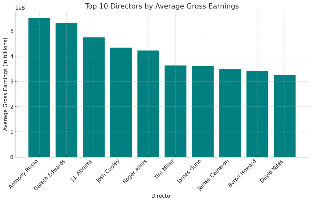
The bar plot above illustrates the top 10 directors by average gross earnings. Directors like Anthony Russo, Gareth Edwards, and J.J. Abrams are associated with some of the highest-grossing films. This visualization emphasizes the significant impact that well-known and successful filmmakers can have on a movie’s commercial success.

Next, let’s visualize the top 5 genres for the top 5 actors by the number of movies they have appeared in, demonstrating their genre preferences:

It seems I made a mistake in the data preparation for the second visualization. Let me correct it and recreate the plot to show the top 5 genres for the top 5 actors by the number of movies they have appeared in.

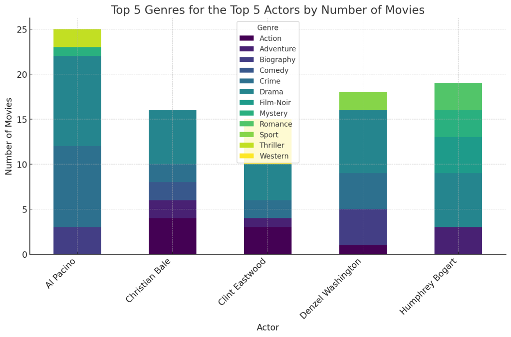
The stacked bar chart above illustrates the top 5 genres for the top 5 actors by the number of movies they have appeared in. It provides a visual representation of the genre preferences of these actors, showcasing their inclination towards specific genres.

For example, we can observe that certain actors have a strong presence in genres like Drama, Crime, and Action, while others have a more diverse portfolio. This visualization emphasizes the relationship between actors and genres, reflecting both personal choices and industry trends.

Together, these visualizations provide a vivid depiction of key aspects of the movie industry, highlighting the influence of directors, the commercial appeal of stars, and the genre affiliations of top actors. They complement our analytical findings, offering a tangible understanding of the dynamics that shape cinematic success and audience reception.

Feel free to reach out if you have any more questions or need further assistance!